K-Nearest Neighbor (KNN) Machine Learning Algorithm

Introduction
A k-nearest-neighbor (KNN) algorithm, is an approach to data classification that estimates how likely a data point is to be a member of one group or the other depending on what group the data points nearest to it are in.
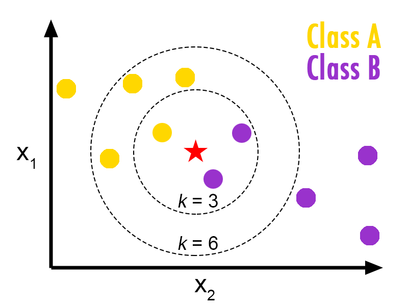
Here’s the basic idea of how k-NN works: suppose there are two different classes, Class A and Class B, in the dataset. Now we have a new data point, which is the red, pentagon-shaped point on the plot below and we want to predict which class this new data point belongs to. When k = 3, there are 2 Class B and 1 Class A in the 3 nearest neighbors of the new data point. The simple majority vote is Class B. Therefore, we predict the new data point belongs to Class B.

To generalize, here are the steps of how k-NN works:
- Getting the labeled data ready
- Pick an appropriate k
- Get the new sample to classify
- Select the k entries that are closest to the new sample
- Take a simple majority vote to pick a category for new sample
Two Parameters of k-NN
Although the k-NN algorithm is non-parametric, there are two parameters we usually use to build the model: k (the number of neighbors that will vote)and the distance metric.
There are no strict rules around the selection of k. It really depends on the dataset as well as your experience when it comes to choosing an optimal k. When k is small, the prediction would be easily impacted by noise. When k is getting larger, although it reduces the impact of outliers, it will introduce more bias (Think about when we increase k to n, the number of data points in the dataset. The prediction will be the majority class in the dataset).
The selection of the other parameter, distance metric, also varies on different cases. By default, people use Euclidean distance (L2 norm). However, Manhattan distance and Minkowski distance might also be great choices in certain scenarios.
Pros and Cons of k-NN
There are multiple advantages of using k-NN:
- It is a simple machine learning model. Also very easy to implement and interpret.
- There is no training phase of the model.
- There are no prior assumptions on the distribution of the data. This is especially helpful when we have ill-tempered data.
- Believe it or not, k-NN has a relatively high accuracy.
Of course, there are disadvantages of the model:
- High requirements on memory. We need to store all the data in memory in order to run the model.
- Computationally expensive. Recall that the model works in the way that it selects the k nearest neighbors. This means that we need to compute the distance between the new data point to all the existing data points, which is quite expensive in computation.
- Sensitive to noise. Imagine we pick a really small k, the prediction result will be highly impacted by the noise if there is any.
Implementation on the Heart Disease dataset
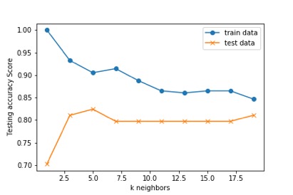
We used KNN as a classifier algorithm. After splitting the heart disease data into train and test sets, the data was scaled and encoded. A KNN classifier model was setup, we looped through a list of K values to determine the best accuracy score.
The results showed that the K=5 results in the best score for both train and test data.

The overall accuracy of the model was 0.784.
Algorithm modification and tuning: Given the limited data samples, K-Fold Cross-Validation was used to resample and evaluate the KNN model.
In k-fold cross-validation, the original sample is randomly partitioned into k equal size sub samples. Of the k sub samples, a single sub sample is retained as the validation data for testing the model, and the remaining k-1 sub samples are used as training data. The cross-validation process is then repeated k times (the folds), with each of the k sub samples used exactly once as the validation data. The k results from the folds can then be averaged (or otherwise combined) to produce a single estimation. The advantage of this method is that all observations are used for both training and validation, and each observation is used for validation exactly once.
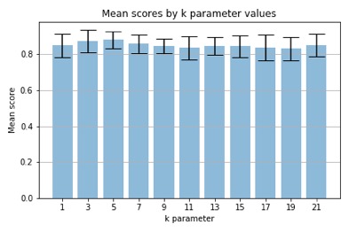
In addition, GridSearchCV along with cross-validation was used to evaluate the model across various parameters.
The graph below shows mean accuracy across the different k values after the k-fold cross-validation and GridSearchCV was used.
