Support Vector Machine (SVM) Learning Algorithm

Introduction
Support vector machine is a simple algorithm that every machine learning expert should have in his/her arsenal. Support vector machine is highly preferred by many as it produces significant accuracy with less computation power. Support Vector Machine, abbreviated as SVM can be used for both regression and classification tasks. But, it is widely used in classification objectives.
The objective of the support vector machine algorithm is to find a hyperplane in an N-dimensional space(N — the number of features) that distinctly classifies the data points.
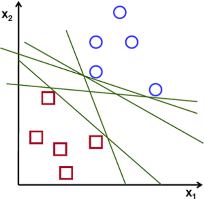
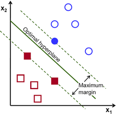
To separate the two classes of data points, there are many possible hyperplanes that could be chosen. Our objective is to find a plane that has the maximum margin, i.e the maximum distance between data points of both classes. Maximizing the margin distance provides some reinforcement so that future data points can be classified with more confidence.
Hyperplanes and Support Vectors
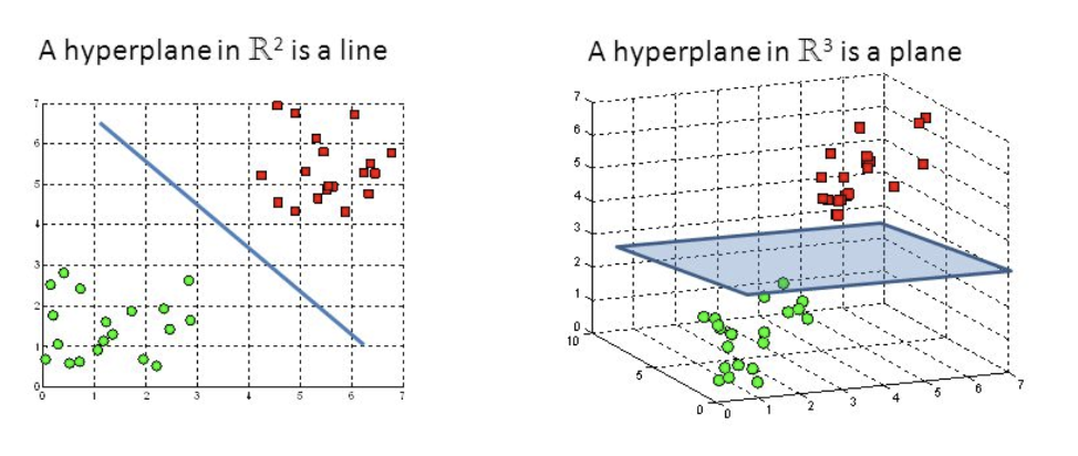
Hyperplanes are decision boundaries that help classify the data points. Data points falling on either side of the hyperplane can be attributed to different classes. Also, the dimension of the hyperplane depends upon the number of features. If the number of input features is 2, then the hyperplane is just a line. If the number of input features is 3, then the hyperplane becomes a two-dimensional plane. It becomes difficult to imagine when the number of features exceeds 3.
Support vectors are data points that are closer to the hyperplane and influence the position and orientation of the hyperplane. Using these support vectors, we maximize the margin of the classifier. Deleting the support vectors will change the position of the hyperplane. These are the points that help us build our SVM.
Implementation on the Heart Disease dataset
The key advantage for the Heart Disease dataset is that SVM is effective for high dimensional spaces. The data set has 13 features (5 variable and 8 categorical). Once the categorical data is reformatted for binary there are 28 features.
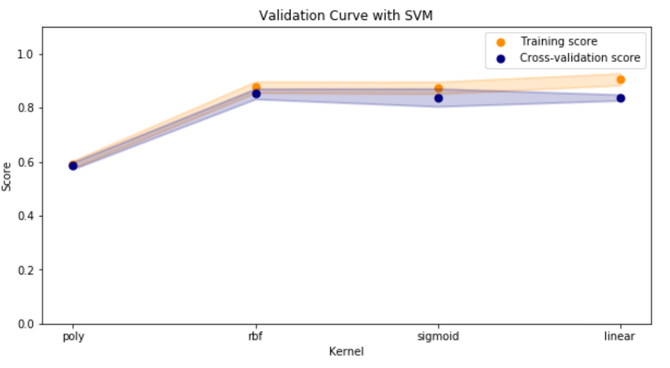
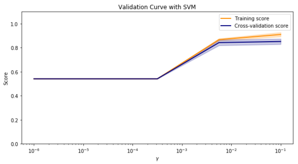
Validation curves were used to visualize and ultimately select the input parameters to maximize the accuracy of the model. A linear kernel was selected and a gamma value of 0.1 to maximize the cross-validation score. The decision function type was irrelevant.
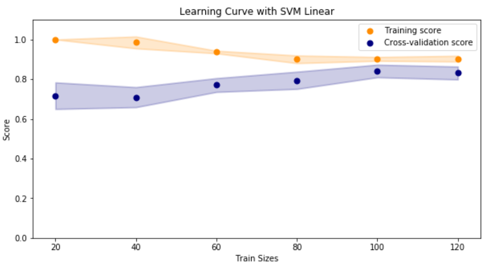
Next, the size of the training set was evaluated using a learning curve. It was confirmed that the default train/test/split method from scikit-learn splits training (220) and testing (74) data sets where the scores converge.
Running the test data set, the following classification report results:

Running this data set on the pre-set train/test split resulted in the following:
- 82% of the time Heart Disease or Healthy was predicted correctly (Accuracy)
- 83% of Heart Disease predictions were Heart Disease (Precision)
- 82% of Heart Disease samples were correctly predicted (Recall)
- Overall 82% harmonic average of precision and recall (F1 Score)