Logistic Regression Algorithm
Introduction
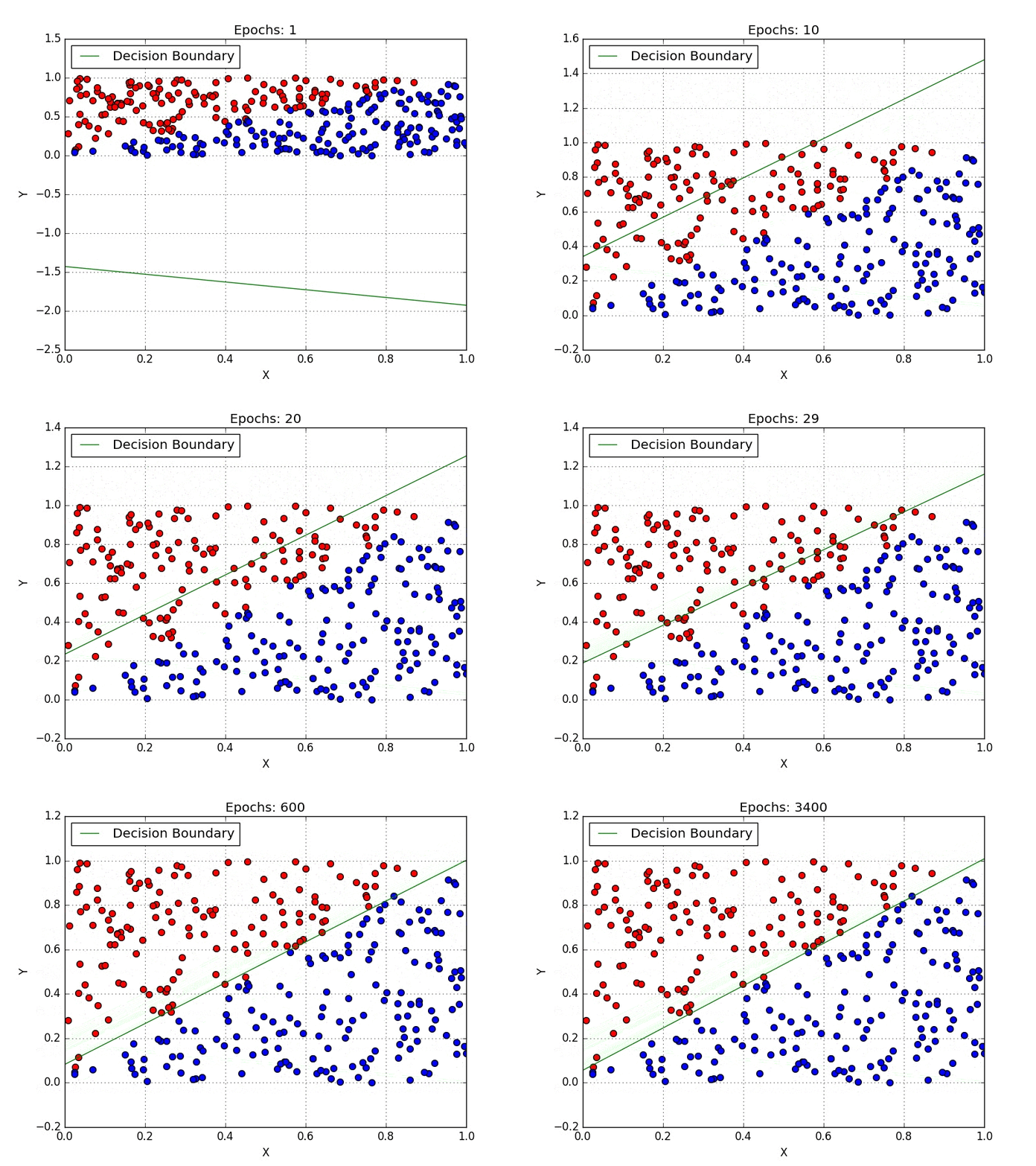
Logistic Regression is a classification algorithm used to assign observations to a discrete set of classes. Some of the examples of classification problems are Email spam or not spam, Online transactions Fraud or not Fraud, Tumor Malignant or Benign. Logistic regression transforms its output using the logistic sigmoid function to return a probability value.
We can call a Logistic Regression a Linear Regression model but the Logistic Regression uses a more complex cost function, this cost function can be defined as the ‘Sigmoid function’ or also known as the ‘logistic function’ instead of a linear function.
The hypothesis of logistic regression tends it to limit the cost function between 0 and 1. Therefore linear functions fail to represent it as it can have a value greater than 1 or less than 0 which is not possible as per the hypothesis of logistic regression.
What is the Sigmoid Function?
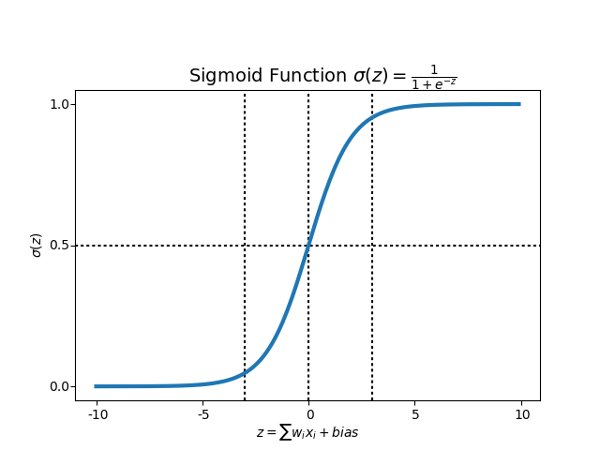
In order to map predicted values to probabilities, we use the Sigmoid function. The function maps any real value into another value between 0 and 1. In machine learning, we use sigmoid to map predictions to probabilities.
Implementation on the Heart Disease dataset
The scikit learn library implementation of Logistic Regression provides multiple settings to tune a model. Using the Heart Disease data set, four settings were tested as follows using a nested for loops to test all combinations a total of 10 times each:
- Tolerances = [0.1, 0.001, 0.00001, 0.0000001]
- Weights = ['balanced','none']
- Maximum Iterations = [10, 50, 100, 500]
- Solvers = ['newton-cg', 'lbfgs', 'sag', 'saga', 'liblinear']
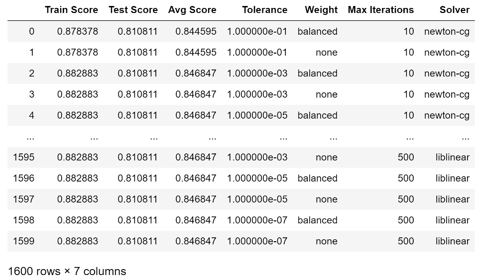
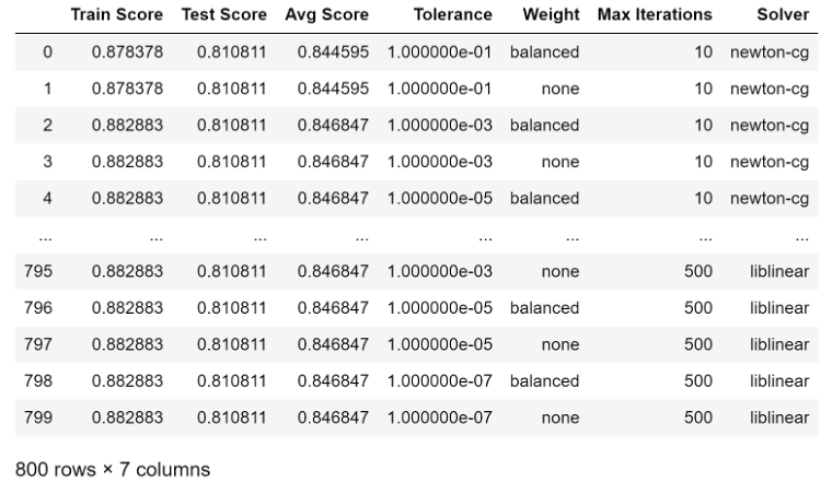
Results were captured and displayed in a data frame:
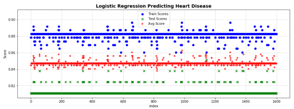
Results were grouped by the four variables and plotted vs the Average Score:
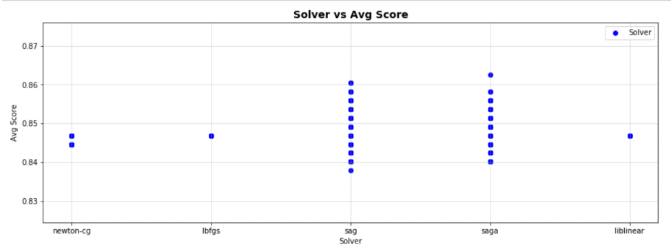
Finally, the max Avg, Train and Test scores were calculated and the data set was reduced to only rows that contain at least one these max values:

These values were then plotted by their index value.
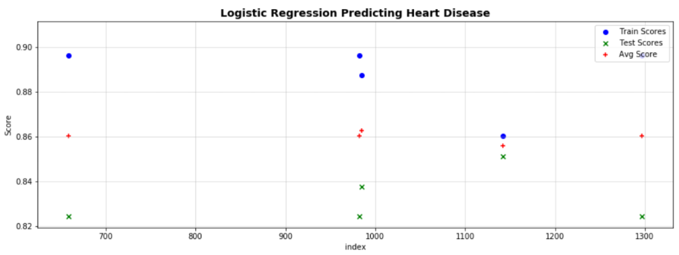
Based on the results, sample 1142 was chosen as it has the most consistent scores for all three and the highest for the Train set.
The following model was then selected:
- Tolerance = 0.0000001
- Weight = 'balanced'
- Max Iterations = 10
- Solver = 'sag'
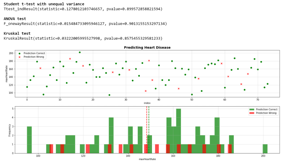
Finally, the test data was run with the new model. The results were broken into ‘same’ (correct) and ‘differences’ (incorrect) populations. They were then plotted vs each variable feature. The mean (ANOVA, Kruskal) and the variation (Student t) of the two populations were checked to ensure they were not different. If they had been, we may have had a problem / opportunity with our model. A sample of the analysis is shown below for max heart rate:
